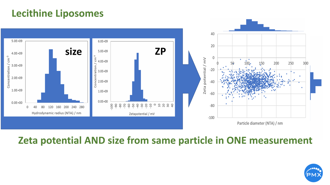
Introduction

ZetaView® tracks the particles individually in a Laser Scattering / Fluorescing Video Microscope. By following the Brownian motion of the particles their diffusion size is deduced^1,2. As soon as an electric field is applied, the particles start an electrophoretic movement. From the unidirectional movement, the electrophoretic mobility µe = v/E is derived, v being the velocity of the particles and E the applied electric filed. With some assumptions, sometimes philosophic, the so-called zeta potential ζ is derived (ZP). When we speak of ZP, it is only about particles moving in a polar liquid like water. This is more than Pareto for the reason, that ZP in any other liquids like organic represents high acrobatic thinking.

The higher the ZP (positive or negative), the higher is the repulsion force between the particles and the lower the probability for a collision with subsequent aggregating. As a simple aid to memory – not always correct – stands “30 mV”. Repulsion is dominant above 30 mV. For the aggregation, the Van der Waals attraction between surfaces is responsible. It starts below 30 mV and increases the nearer zeta potential approaches zero.

Literature

All this is written in detail first by famous scientists like Smoluchowski, Einstein, Stokes and colleagues, later by Hunter, Lagally and others. An excellent description is given in the ISO documents 13099:2008, part 1 (general) and 2 (optical methods). Part 3 (organic solvents) is in preparation. ASTM_E2834-12 is the corresponding American Standard. For literature references we recommend again the mentioned standard publication. Articles In simpler depiction you may find in our home page.

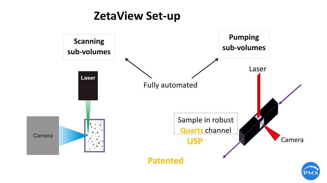
Focus position control for the micro- electrophoresis set-up in the Particle Metrix ZetaView®

In a 90° scattering/ fluorescing microscope like ZetaView®, the electrophoretic mobility measurement is accompanied by the electro-osmosis effect. Electro-osmotic flux of the medium is a reaction of the mobile counter- ions in the liquid to the electric field. These counter ions carry a charge opposite to the cell wall. The electro-osmosis therefore reflects the polarity and amount of the ions sitting on the surface of the wall. The migrating ions drive the whole liquid, with the liquid also the suspended particles. Electrophoresis and electro-osmosis motion superimpose each other. The separation of both effects is possible only in the so-called “stationary layers”, where electro-osmosis is zero. These layers are shown by the 2 dashed vertical lines in Fig. 4 of the brochure (see below).

From looking to the velocity (here zeta potential) profiles of the liquid in figure 4, it is clear, that the location of the combined focus of the laser and the microscope must be controlled over the entire cross section of the cell. Scanning from one side (wall 0) to the other side (wall 1) is a must. The velocity profile is recorded and the electrophoretic mobility (zeta potential) taken from the 2 stationary layers. Particle Metrix takes full control of it. The user has not to take care about electro-osmosis influences.

If the sample is very salty like a sample in PBS, convection may occur. To avoid this, the field is alternated at a sufficiently high repetition rate, so that the electrophoretic motion of the particles is measurable, whereas the motion of the total sample due to electro-osmosis cannot follow.

This scan helps not only in zeta potential analysis but is useful also to guarantee statistically valid size and concentration analyses by measuring concentration and size at all the 11 stops during a cell profile scan. The automatic measurement is shown below:

<pProgramming a kinetic measurement where each profile scan is followed by a burst of 5 µl new sample, the statistical validity is boosting. See the next slide (or Video):</p>

How to measure the size and electrophoretic component of an individual particle simultaneously?

A SOP starts the zeta potential measurement at the stationary layers. The rest is mathematical separation of the uni-directional electrophoretic movement from the random Brownian motion. This is documented as a scatter plot below.

The following example shows the kinetics of zeta potential and size after adding 2 mM NaCl solution to a dispersion of 40 nm gold particles.

The kinetics is programmed in 2 steps, first by scanning 11 positions and, if wanted, second by pumping a new sample. 

Zeta potential experiments are possible in the scattering and fluorescent mode of the ZetaView® NTA.

ZP vs size Scatterplot in fluorescence mode

As an example